이 책의 모든 코드는 깃허브로 제공됩니다. (https://github.com/rickiepark/handson-ml3)
책의 설명대로, 블로그 글은 구글 코랩을 활용해 진행하겠습니다. (https://colab.research.google.com/github/rickiepark/handson-ml3/blob/main/)
1. 데이터 다운로드 및 확인
1.1 데이터 다운로드
from pathlib import Path
import pandas as pd
import tarfile
import urllib.request

def load_housing_data():
    tarball_path = Path("datasets/housing.tgz") 			# datasets/housing.tgz 파일을 데이터로 가져옴
    if not tarball_path.is_file():					# 실패할 경우, is_file은 해당 경로가 파일인지 확인, 파일이면 True, 아니면 False
        Path("datasets").mkdir(parents=True, exist_ok=True)		# pahtlib을 활용해 datasets라는 디렉토리를 만듦, mkdir=make directory, parents=True 상위 디렉토리가 없으면, 상위 디렉토리도 생성, exist_ok=Ture datasets이 존재해도 오류없이 그대로 진행
        url = "https://github.com/ageron/data/raw/main/housing.tgz"	# url 변수로 데이터가 저장된 온라인 주소를 가져옴
        urllib.request.urlretrieve(url, tarball_path)			# urlib.request = URL을 열고 데이터를 가져오는 lib, .urlretrieve = URL에서 파일 다운로드, urlretrieve(url 주소, 저장할 파일 이름)
        with tarfile.open(tarball_path) as housing_tarball:		# with문 사용(아래서 따로 설명)
            housing_tarball.extractall(path="datasets")
    return pd.read_csv(Path("datasets/housing/housing.csv"))		# 경로에 있는 데이터를 반환함

housing = load_housing_data()						# 반환된 데이터를 housing에 저장
with 문 설명
# with문

# with문은 as와 함께 사용
# DB을 열거나 파일스트림과 같이 사용하기에 편리함
# 마지막에 close을 하지 않아도 됨

# with문 형식
with open('file.txt') as data:
	print('success')
# file.txt을 열어서 data라는 변수로 저장해준다. 성공하면 success을 출력.

# 따라서 위의 코드를 해석해보면,
        with tarfile.open(tarball_path) as housing_tarball:
            housing_tarball.extractall(path="datasets")
        # 이전 코드에서 tarball_path에 데이터의 경로를 담아둠
        # 데이터의 경로에서 파일을 열어 housing_tarball에 저장
        # extractall() = 파일 내부의 모든 압축파일을 압축 해제
        # housing_tarball의 모든 압축파일을 압축 해제하여, datasets에 저장
1.2 데이터 확인
housing.head()					#데이터를 표로 확인, 처음 5행만
housing.info()					#데이터 타입, column등을 확인
housing["ocean_proximity"].value_counts()	# housing의 column중 ocean_proximity 값의 개수(value_count)을 확인
housing.describe()				#describe는 숫자형 특성의 요약 정보를 제공 (count, mean, std, min 등등)
1.3 추가 코드 (고해상도 이미지 저장)
저장하기 위한 함수를 지정
# 추가 코드 - 고해상도 PNG 파일로 그래프를 저장하기 위한 코드

IMAGES_PATH = Path() / "images" / "end_to_end_project"				# 기본 path 밑에 images\end_to_end_project 경로를 생성
IMAGES_PATH.mkdir(parents=True, exist_ok=True)					#디렉토리를 만들고, 상위 디렉토리가 없으면 만들고(parents=True), 파일이 이미 존재해도 에러 없이 진행(exist_ok=True)

def save_fig(fig_id, tight_layout=True, fig_extension="png", resolution=300):	#함수 선언, fig_id만 받고 나머진 고정값으로 지정됨
    path = IMAGES_PATH / f"{fig_id}.{fig_extension}"				# IMAGE_PATH 경로 아래에 fig_id.fig_extension(png)로 저장
    if tight_layout:
        plt.tight_layout()
    plt.savefig(path, format=fig_extension, dpi=resolution)			# path에 이미지를 저장

# 저장만 할뿐, 반환할 것이 없기때문에 return은 없음.
1.4 데이터 plot
import matplotlib.pyplot as plt

# 추가 코드 – 다음 다섯 라인은 기본 폰트 크기를 지정합니다
plt.rc('font', size=14)
plt.rc('axes', labelsize=14, titlesize=14)
plt.rc('legend', fontsize=14)
plt.rc('xtick', labelsize=10)
plt.rc('ytick', labelsize=10)

housing.hist(bins=50, figsize=(12, 8))
save_fig("attribute_histogram_plots")  # 추가 코드
plt.show()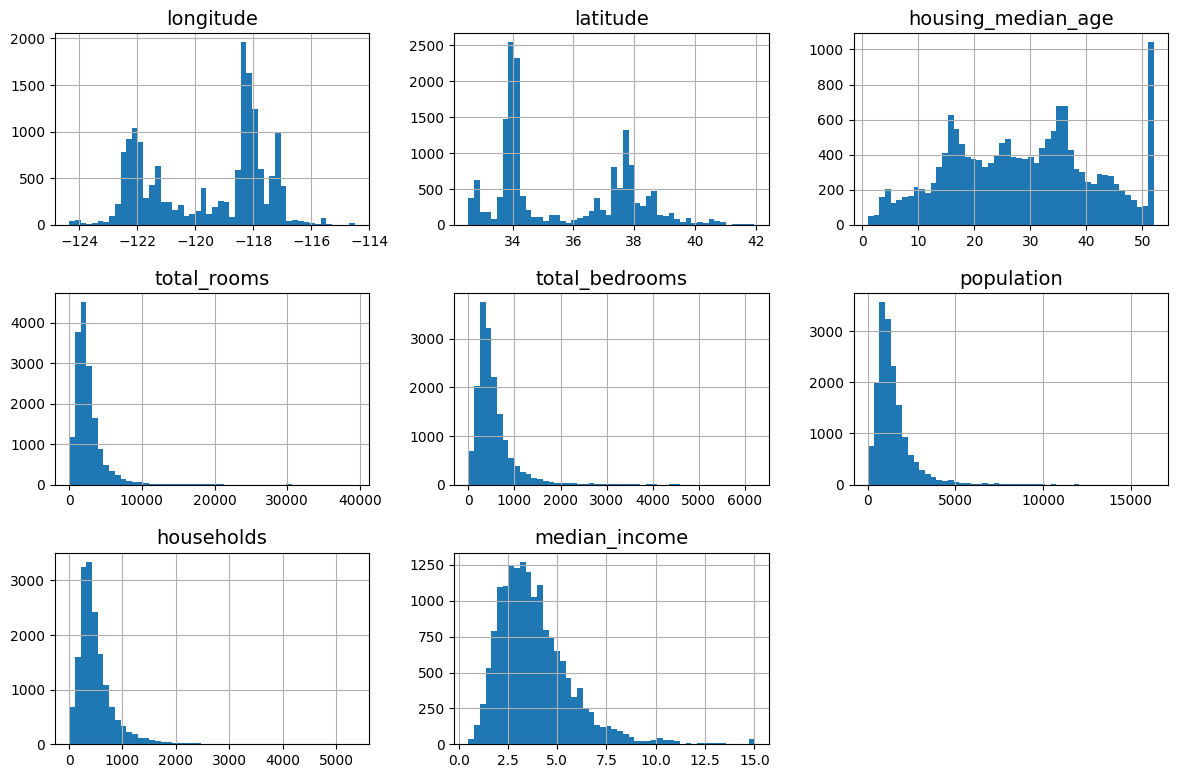
2. 테스트 세트 만들기
2.1 Training set과 test set 나누기
import numpy as np

def shuffle_and_split_data(data, test_ratio):			# 데이터(data)와 테스트 세트로 활용할 비율(test_ratio)을 받음
    shuffled_indices = np.random.permutation(len(data))		# np.random.pernutation에 데이터의 크기(len(data))을 넣으면, 랜덤한 n개의 수가 얻어짐
    test_set_size = int(len(data) * test_ratio)			# 데이터 셋의 크기는 전체 데이터에서 비율을 곱한 값을 사용
    test_indices = shuffled_indices[:test_set_size]		# 섞은 데이터에서 1번째부터 test_set_size까지는 test 셋으로 사용
    train_indices = shuffled_indices[test_set_size:]		# 섞은 데이터에서 test_set_size부터 마지막까지는 train 셋으로 사용
    return data.iloc[train_indices], data.iloc[test_indices]	#전체 데이터에서 각 세트에 맞는 데이터를 슬라이싱해서 반환
마지막 return 부분에서 이해가 안 되었지만, len으로 각 데이터의 번호를 매기고, shuffle로 섞은 다음, indice에서 번호에 따른 데이터 셋을 지정하는 방식
아래에 간단히 예시를 보면,
# 코드 이해를 위한 예제
data = [1,3,2,4,7,6,8,10,11,26,34,88,125,679]
data = pd.DataFrame(data)
test_ratio = 0.2

test_set_size = int(len(data) * test_ratio)		# 결과 : 2
shuffled_indices = np.random.permutation(len(data))	# 0부터 전체 데이터 개수(13)까지 수를 랜덤하게 섞음 (index을 섞는것)
shuffled_indices					# 결과 : array([ 5,  3,  2,  8,  1, 10,  4, 11,  0,  9,  7,  6, 13, 12])
test_indices = shuffled_indices[:test_set_size]		# 결과 : array([5, 3])
train_indices = shuffled_indices[test_set_size:]	# 결과 : array([ 2,  8,  1, 10,  4, 11,  0,  9,  7,  6, 13, 12])
# 앞에서부터 test_set_size까지는 test 셋으로, 나머진 train 셋으로 구분됨

data.iloc[train_indices]
# 결과
#   0
# 2	2
# 8	11
# 1	3
# 10	34
# 4	7
# 11	88
# 0	1
# 9	26
# 7	10
# 6	8
# 13	679
# 12	125

data.iloc[test_indices]
# 	0
# 5	6
# 3	4

#각 index 번호에 맞는 데이터가 train과 test 셋으로 분류됨
하지만 위 함수는 업데이트된 데이터 셋을 활용할때 문제가 생김.
트레이닝 셋과 테스트 셋이 매번 섞임
이에 데이터마다 고유한 식별자를 사용해서 데이터셋이 경신되더라도 테스트/트레이닝 셋이 동일하게 유지되게 해야 함.
아래에서 이를 구현
from zlib import crc32

def is_id_in_test_set(identifier, test_ratio):
    return crc32(np.int64(identifier)) < test_ratio * 2**32
    	# crc32는 해쉬값을 만들어주는 함수
	# np.int64는 identifier을 64비트 정수로 변환해줌 (crs가 정수 타입을 요구)
        # 이후 crs32을 통해서 해쉬값을 만들게 되면, 범위는 0에서 2^32-1의 범위를 가짐
        # 여기에 test_ratio을 곱해서 작으면 test 세트에 포함해 반환, 아니면 반환하지 않음( training 세트)

def split_data_with_id_hash(data, test_ratio, id_column):
    ids = data[id_column]		# data의 id_column을 ids로 저장
    in_test_set = ids.apply(lambda id_: is_id_in_test_set(id_, test_ratio))
    	# labda는 def와 동일한 효과, lambda 입력변수 : 리턴값으로 구성됨
        # id_을 앞에서 정의한 is_id_in_test_set에 넣어서 값을 리턴함
    return data.loc[~in_test_set], data.loc[in_test_set]
데이터셋에 식별자 컬럼이 없으므로,. reset_index()을 통해서 추가해 줌
. reset_index() 함수
주요 인자
drop
drop=False일 경우, 기존 인덱스가 데이터프레임의 새로운 열로 추가됩니다. (디폴트)
drop=True로 설정하면 기존 인덱스 열을 삭제하고 인덱스만 리셋됩니다.
inplace
inplace=False로 설정하면 새로운 데이터프레임이 반환되며, 원본 데이터프레임은 변경되지 않습니다. (디폴트)
inplace=True로 설정하면 원본 데이터프레임이 직접 변경됩니다.
housing_with_id = housing.reset_index()  					# 원본 데이터는 수정하지 않고, 원본 데이터에 `index` 열 추가해서 새로운 변수에 저장
housing_with_id["id"] = housing["longitude"] * 1000 + housing["latitude"]	# 고유 식별자를 만들기 위해, 구역의 위도와 경도 값을 활용
train_set, test_set = split_data_with_id_hash(housing_with_id, 0.2, "index")	# 새로운 방법으로 데이터 나눔
사이킷런을 활용해도 괜찮음
이 함수는 이전에 정의한 shuffle_and_split_data() 함수와 유사하게 작동함.
# 사이킷런을 활용한 방법

from sklearn.model_selection import train_test_split

train_set, test_set = train_test_split(housing, test_size=0.2, random_state=42)
2.2 계층화
주택 가격을 예측하는 프로젝트 특성상, 중간 소득이 매우 중요하다고 가정할 경우.
이때 소득별로 계층화해서 별도 레이블을 부여해야 함
유용한 함수가 pd.cut 함수
pd.cut(데이터, bins=나눌 구간, label=지정할 레이블)
housing["income_cat"] = pd.cut(housing["median_income"],
                               bins=[0., 1.5, 3.0, 4.5, 6., np.inf],
                               labels=[1, 2, 3, 4, 5])
계층 분할에 있어 사이킷런의 train_set_split 함수를 사용해도 괜찮음
from sklearn.model_selection import StratifiedShuffleSplit

splitter = StratifiedShuffleSplit(n_splits=10, test_size=0.2, random_state=42)
	# n_spllit = 반복해서 나눌 횟수, test_size = 테스트 세트의 비율, random_state = 난수 생성의 시드

strat_splits = []
	# 빈 리스트를 만들어 저장하기 위함

for train_index, test_index in splitter.split(housing, housing["income_cat"]):
    strat_train_set_n = housing.iloc[train_index]
    strat_test_set_n = housing.iloc[test_index]
    strat_splits.append([strat_train_set_n, strat_test_set_n])


strat_train_set, strat_test_set = train_test_split(
    housing, test_size=0.2, stratify=housing["income_cat"], random_state=42)

    # train_set_split(분할할 데이터프레임, 전체 중 테스트 세트로 사용할 비율, 기준으로 삼을 열, 난수 생성 시드(없으면 매번 다름, 같은 숫자를 지정하면 매번 동일)
계층으로 샘플링한 것과 랜덤 샘플링의 결과를 비교해 보면, 계층 샘플링의 오차가 확실히 작은 것을 알 수 있다.
# 비교를 위한 함수 정의
def income_cat_proportions(data):
    return data["income_cat"].value_counts() / len(data)			# data에서 incom_cat의 비율을 계산

train_set, test_set = train_test_split(housing, test_size=0.2, random_state=42)

compare_props = pd.DataFrame({
    "Overall %": income_cat_proportions(housing),				# 전체데이터
    "Stratified %": income_cat_proportions(strat_test_set),			# 계층적 분할
    "Random %": income_cat_proportions(test_set),				# 무작위 분할
}).sort_index()														# 데이터 정렬
compare_props.index.name = "Income Category"
compare_props["Strat. Error %"] = (compare_props["Stratified %"] /
                                   compare_props["Overall %"] - 1)
compare_props["Rand. Error %"] = (compare_props["Random %"] /
                                  compare_props["Overall %"] - 1)
(compare_props * 100).round(2)							# 각 데이터에 100을 곱하고 소수점 두 자리로 반올림
| Income Category | Overall % | Stratified % | Random % | Strat. Error % | Rand. Error % |
| 1 | 3.98 | 4.00 | 4.24 | 0.36 | 6.45 |
| 2 | 31.88 | 31.88 | 30.74 | -0.02 | -3.59 |
| 3 | 35.06 | 35.05 | 34.52 | -0.01 | -1.53 |
| 4 | 17.63 | 17.64 | 18.41 | 0.03 | 4.42 |
| 5 | 11.44 | 11.43 | 12.09 | -0.08 | 5.63 |
2.3 데이터 plot
housing["income_cat"].value_counts().sort_index().plot.bar(rot=0, grid=True)
	# incom_cat 데이터를 value_count()로 개수를 카운트
	# sort_index() - 레이블이 정렬이 안되있으므로, 정렬해줌
	# plot.bar(rot=0, grid=True) - 막대 그래프로 시각화, x레이블의 회전 각도는 수평, grid 생성
plt.xlabel("Income category")
plt.ylabel("Number of districts")
save_fig("housing_income_cat_bar_plot")  # extra code
plt.show()
'공부 > Python' 카테고리의 다른 글
| [핸즈온 머신러닝] Ch.2 머신러닝 프로젝트 처음부터 끝까지 - 2(2.4) (1) | 2024.09.05 |
|---|---|
| [핸즈온 머신러닝] Ch.1 머신러닝 기초 배경 (1) | 2024.09.03 |
| [Python 기초] 기타 함수 (enumerate, zip, lambda, map) (0) | 2024.08.26 |
| [Python 기초] 예외처리 (try, except) (0) | 2024.08.25 |
| [Python 기초] 함수, Global (0) | 2024.08.24 |